
In this video, Corey describes the design profile of worm gears and how they are used in industry.

Check this Out
In this video, Corey describes the design profile of worm gears and how they are used in industry.
Springs are essential to life. In fact everything on the planet acts like a spring, which follow Hooke’s law. When force is applied to an object, it will deflect. If more force is applied, it will deflect more.
When designing or selecting a compression spring the following items need to be considered:
One crucial thing to understand when designing compression springs is to be sure to operate them in their intended range. All springs work well in their linear range, but as soon as they are loaded past the yield strength, the spring stops behaving as intended and the spring life is severely shortened. It is little known that springs are one of the most energy efficient methods of storing energy as very little heat is created in the process.
One of the most fascinating things about springs is that the method they are used in is opposite of the load they see. A compression or extension spring is loaded in torsion and a torsion spring is loaded in bending. I liken this to driving on parkways and parking on driveways. It’s all backward!
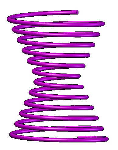
Cylindrical compression springs are by far the most common, but there are other shapes to consider. The most popular are:
Cylinderical springs are very common and come in a variety of sizes as an off the shelf part. The OD and ID of the spring is consistent and as a result, they are generally intended to be guided by being placed in a bore or over a shaft. The spring rate is constant and adding springs in series will enable more travel, while adding them in parallel allows for more force.
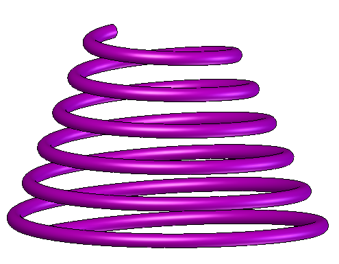
Conical springs are widely used as well. They are prevalent in most battery powered electronics as they squeeze the negative terminal of the battery and hold it in place. A conical spring has a constantly decreasing radius. The main reason to use this type of spring is height constraint; the coils will nest inside each other until the collapsed height is roughly two thickness of the wire diameter. This allows more stored energy in a smaller space. Because the diameter of the spring is not constant, the spring rate is non-linear. When you push on a conical spring, the outer coils will compress first and the spring rate will continually increase as the diameter decreases. Conical springs also have some tolerance for lateral movement as one would see when a battery is inserted into the electrical device with a slight offset from the battery center-line. Along with hourglass and barrel springs, conical springs are often chosen when spring surge is an issue.
Hourglass Springs are nose to nose conical springs. They allow for high loads in small heights. The main reason to choose an hourglass spring is for lateral stability. To demonstrate this, imagine holding the spring between the flat palms of your hands. If I push my hands together, I compress the spring. If I keep my hands parallel and the same distance apart, but shift them side to side, I add lateral loads. An hourglass spring will naturally resist this motion because of its wide base and shape. This is the reason that these springs are used in the railroad industry.

Barrel springs are used when buckling is an issue. Sometimes, to get the load capability needed the spring becomes very tall. If there is not a bore the spring fits into or a shaft it fits over, normal springs will buckle. A barrel spring has narrow ends and a much wider center. The wider middle section gives it more stability against buckling.
The second reason to use a barrel spring is it can be designed to reduce the total height just like a conical spring. Once again, the spring rate is non-linear.

The final type of spring is a reduced end spring. You would select one of these for the same reason as a barrel spring. The main difference is that the reduced end spring is far more linear in nature.
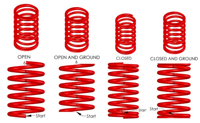
There are four basic types of compression spring ends, they are:
An open end spring will have wire cut perpendicular and none of the coils touch each other in the relaxed state. The pitch is consistent throughout the length of the spring. An open and ground spring is different because the wire is ground at each end so that the spring can lay flush and not leave an indent in whatever it mates to. However, due to the nature of the open spring, there isn’t much material ground off the part.
A closed spring will have the last two coils touching. This offers more support at the end, but it will shorten the number of active coils by two thus changing the spring’s characteristics. They are also available in closed and ground versions so that they can lay flush.
Even if the ends of a spring are ground, they are not and cannot be perfectly perpendicular. As the spring is compressed, the ends will deform angularly thus causing the spring end to rock on a flat surface. This can lead to unevenness in the spring constant thus rendering it a variable defined by its height. In most cases, the application is not critical enough and the average spring rate can be used.
If this is an issue in your application there are two remedies to minimize the effects. Change the end of the spring from an open to a closed condition. As you can see from the diagrams, an open and ground spring will only have a small part of the spring ground. The closed condition grinds a large percentage of the last coil off and therefore offers more support to the end of the spring. If your wire diameter is smaller than 0.20” this will most likely solve your problem.
The other solution is to specify that the spring be ground at a specific height or load applied. This is a custom spring and you will pay for the vendor’s extra attention.
Counting the number of coils on a spring can be tricky. There are two variables that specify the number of coils. The value Na is the number of active coils and Nt is the total number of coils. Only in the case of an open spring is Na equal to Nt.
First of all, you cannot count any coils where the coils are closed or touching. These are inactive coils which don’t cause the spring to be a spring. Start counting each coil from one end to the other starting where the section first opens. For an open end spring, this is the first coil. Keep counting until you get to the other end of the spring. Generally speaking, coils are counted as full turns, but half and quarter turns are also widely used. Many spring manufactures will allow two digits of precision on the number of coils. For torsion springs, like clothes pins, you will specify the end condition in degrees.
In the examples shown, each spring has 6 coils even though the closed end spring has 8 total coils. The table below shows the relationship between active coils, total coils, the solid height and the pitch of each spring type. Allow a 3% tolerance on the solid height to account for the end conditions, wire diameter tolerance and helical wind waviness.

Some springs need to be “set” so that there is a uniform initial or relaxed height. For compression springs, the spring is “set” or “take a set” to the correct height when it is compressed for the first time. To do this, compress it to its collapsed height and release. As you can imagine, the setting process will leave the spring height shorter. At this point the spring will have been set and it will return to this height every time as long as the loads are within the springs limits.
For standard springs, this is done at the manufacturer so they can provide consistent product and not have to deal with the question, “Why are my springs too tall?” from every customer.
However, if you are ordering a custom spring, the vendor may not be able to (or just not want to) set your spring. If this is the case, you have two options. Option 1: you can assemble the spring and let the first operation set the spring. This may work in some cases, but if the application doesn’t compress the spring enough or if the spring won’t physically fit option two is needed.
Option 2: set the springs yourself. For small springs, you can simply squeeze them in your hands. For larger springs, you may need a pneumatic or hydraulic press. This can be a very time consuming process. When designing a custom spring, be sure to consult your vendor for how much set is expected so that you can design your spring to be taller when wound and the right height when set. Your vendor should have plenty of data to get you an accurate spring design.
All springs function according to their dimensions. The dimensions will specify the stresses seen in the spring. Based on general stress calculations, we know that the largest stresses in a compressive spring will be on the outside surface of the wire as load is applied.
When designing a spring, the dimensions are critical to spring characteristics. Often we are confined by the form factor where the spring is applied, i.e., the spring needs to fit in a ¾” hole or over a ½” rod. As the designer, if you find that there is only one or two choices for springs available, you may want to ask yourself if you are being too strict with the design. I have often found that in my design I needed to go up in capacity, but the form factor was already set in stone. Now it is really hard to get the performance I need. Had I adjusted my design to have four or five choices of springs, I could simply change out a spring. In practice, I desire to have five choices; my ideal spring plus two stronger and two weaker spring alternatives.
The life of the spring is dictated by fatigue. As the spring is cycled, grains in the steel rub against each other. As they repeatedly rub, small cracks will get larger and larger until failure occurs. There are two main components that dictate the life of a spring; the number of cycles and the stress intensity.
The number of cycles is pretty easy to determine, it is something that is easily counted or estimated. We find that most materials have an endurance limit, where if the spring makes it to that number of cycles, it will last forever. For steel, this occurs around 1-2 million cycles. Unless your spring is custom, vendors only make springs with infinite life. Even then, vendors will fight you on a finite life spring.
Stress intensity is much more complicated. A lot of it has to do with the mean (average) and alternating stresses. The average stress, alternating stress and stress range are defined by the following equations. We will use a maximum stress of 50 ksi and minimum stress of 10 ksi.
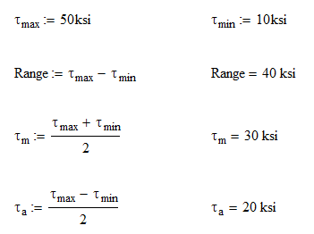
Since we are only dealing with compression springs, the minimum stress is usually zero unless the spring is always compressed. In the case above, we will always have a preload on our spring. This is usually the case in applications where a handle needs to be centered. We want preload on it so that the handle doesn’t vibrate when at rest and it also requires some force to move when leaving the center position. (They are also a pain to install as well.) In any case, our stress range is 40 ksi. To extend our spring life, we will want to decrease this as much as possible. If a spring was to be used as both an extension and compression spring, the minimum stress would be negative thus increasing the stress range greatly and decreasing life span.
One step that spring manufacturers perform to limit the magnitude of stress is to stress relieve. The stress relieving process heats the spring to high temperatures so that permanent or residual stresses from the forming process are eliminated. The temperature here is not so high that the spring would lose its initial temper.
There are generally three different categories that spring design fits in to:
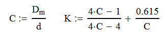
The spring index is a simple ratio of the mean diameter to the wire diameter. It is a variable used in many spring calculations and give us an idea of what type of spring it is. The index should be kept between 4 and 10.
If it is lower than 4 and your spring is coiled too tight, this will require special tooling to form. When forming a tight radius, you might also have problems with the material cracking internally and that will lead to premature failure.
Spring indexes greater than 10 means the spring will be real flimsy and lead to problems with packaging and tangling. Think of a slinky. You also won’t be able to grind or perform other operations like plating.
This should be a giant red flag that something is not right with your design. Don’t design yourself into a hole!
So this is a little bit of a backwards approach. There are five main ways of selecting a spring, but they only make sense once you understand the equations behind spring design. For this we will go through the calculations and then come back to the methods of selection.
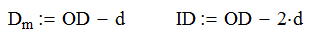
Most spring design is done based on dimensions so it is likely that you will have the outside diameter (OD) and the wire diameter. From these two pieces of information, we can find the inside diameter (ID) and the mean diameter, Dm using the following equations:
From here we can calculate the stress on the spring (assuming the wire is round).
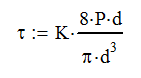
Where C is the spring index, P is the applied load and K is the stress concentration factor. Note K is shown for extension and compression springs. Other types of springs have different values.
The final step is to calculate the spring rate, R
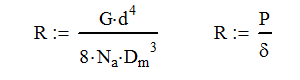
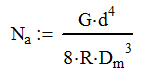
Where G is the shear modulus of elasticity and δ is the deflection. Many times you will be given the spring rate, so we can rearrange this equation to calculate the number of active coils in the spring.
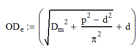
The last thing that you may want to know about your compression spring is how much it expands as it is loaded. This is important to know if your spring is compressing in a bore or extending over a rod. At the solid height (SH), the diameter is defined as:
There are five basic methods for selecting a compression spring. You will need to select one of the five that best fits your application.
Case 1: Design based on physical dimensions
This is probably the most common method of designing a spring. When approaching the design you probably already have a certain envelope that the spring must fit into or around. When selecting a spring by physical dimensions, you need to specify two of these three things:
Case 2: Design based on spring rate
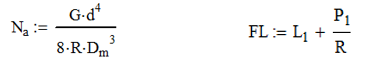
When you know the spring rate you desire, you can start your selection there. You will need other information such as free length, load capacity or some dimension of the spring to complete the selection. Once you have selected this information you will probably be able to calculate the number of active coils and the free length using the following equations.
Case 3: Design based on two loads
For this design criteria, you will specify the spring rate based on two loads that are applied to the spring. At each load, the spring will deflect differently. Many spring manufacturers will have this option of choosing a spring on their website. The variable, L, is the total height of the spring and not the deflection.
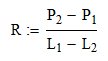
(Note: Spring rates are always positive. Swap L1 and L2 if needed). Once you have the rate, you are basically back in the previous design case (Case 2) and need to make other decisions to select your spring.
Case 4: Design based on one load and spring rate
This is really another subset of load Case 2. The only difference is we will be able to calculate the free length without making any other selections.
Case 5: Design based on one load and free length
This is really just a subset of Case 3 where we assume that P2 is 0 lb and L2 is the free length. Then use the equations in Case 2.
I need a spring that will fit in a 1.25” hole and have a free length of 5.00 in. I need a spring that will support at least 100 lb without bottoming out. I then go to Lee Spring’s website and search for what I know: fits in 1.25” hole and free length of 5.00 in. I get the following results.

Looking through the list, I have multiple options which means that my design is reasonable and I’m not designing myself into a corner. I look through the spring rate column and notice that the first four springs are just not going to cut it. A spring rate of 5.3 lb/in is going to take 20” of compression to get me to 100 lb! The 22.25 lb/in spring rate is probably just outside of where I need to be. I have selected the 53 lb/in spring as a starting place because my deflection at 100 lb will be just less than 2”. At this time, I will perform my hand calculations (left) and determine the results. I have also displayed the additional information from the manufacturer (right). Notice how my calculations of solid height, active and total coils match with the manufacturer. We also have a maximum load capability of 140 lb. I have also added a calculation for W which is the working range of the spring. I’m not sure why manufacturers don’t provide this, but it would be nice.
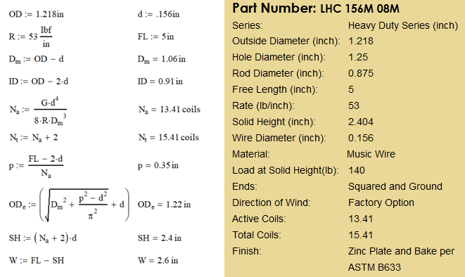
At this point, we can move on to the stress calculations for this spring. Since we are using music wire, we will assume that for this diameter, the tensile strength is 225 ksi.
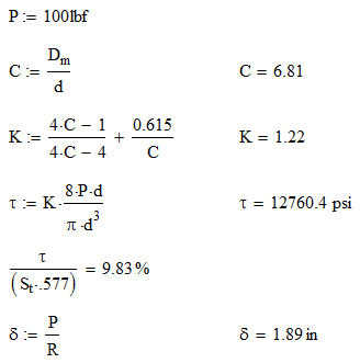
As you can see from the stress calculations, the intended load is only 10% of the tensile strength. Also, our deflection is 1.89 in as we estimated. If you are curious as to where the 0.577 comes from, please watch the video on Mohr’s Circle.
Spring design seems complicated because there are so many different ways to approach it. Just remember that there is no perfect solution for your application. With all the off-the-shelf sizes, shapes and materials to choose from, you will select a very good spring for your application. Just remember to watch for the red flags of improper spring index and always have plenty of alternative springs ready.
You got this!
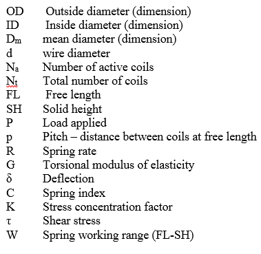
Glossary of Terms
In this video, Corey describes how differential gears work. He also explains how limited slip differentials get you out of the mud.
One common task for a design engineer is to design an articulating system. Often this is for lifting objects as is the case with a crane, aerial lift platform or even my log splitter’s jib. Cylinders are a great choice for powering this articulation because they are able to provide large amounts of force in a small package. The task of designing an articulating boom seems daunting, but with the advent of 3D CAD, MathCAD and/or Excel, the job has been simplified.

In order to layout the geometry for an articulating cylinder you will need to determine the articulation range and then lay it our in 3D CAD using a parametric sketch. Create a mathematical model that will calculate to loads and forces needed for the geometry. Finally, select a cylinder and tweak the design.
Let’s investigate each step a little deeper.
This is by far the most critical step, but it is often overlooked. In order to properly design a system that is robust, you need to have a firm grasp on the reach and height requirements. Loading should also be considered here too. Failure to do this often results in having a machine that needs to be ‘stretched’ to meet customer demands. Stretching a unit is never a fun thing and it leads to a patched design at best or complete rework at worst.
For a single cylinder articulation design, 120° of
articulation is the maximum you want to plan on. The articulation is really pushing it at
125°, but don’t go there unless absolutely necessary. The reason is that 5° more articulation
really cuts down on your moment arm for the cylinder; this requires a larger
cylinder. Another less noticeable
downside is the articulation speed will be really fast at either end, but slow
at mid-cylinder stroke. If you need
articulation greater than 120°, linkage and/or a second cylinder may be
needed. Linkage, sometimes referred to
as ‘four bar linkage’ is a method of improving the articulation angle. Instead of having one end of the cylinder
connected directly to a structure, it will pin with four links. The links are designed such that it will keep
the cylinder far enough away from the boom creating a good moment arm
throughout the articulation. The subject of linkage for articulating designs is
vast and we will need to discuss that in a future article.
The advent of 3D CAD and parametric sketch drawing has made this step a breeze! When I was a young engineer, I once witnessed an older colleague who was laying out a cylinder in AutoCAD. This was a very hard thing for me to watch as he spent the greater portion of a day trying to find favorable cylinder geometry. Since AutoCAD is non-parametric, every change in mounting location or cylinder length lead to multiple move and rotate commands. Having just been trained in Solidworks, I knew that technology would greatly reduce the complexity and time it takes to come up with good cylinder geometry. It was on that day that started developing the method I am sharing now and have been using for fifteen years. In this process we will demonstrate how we can use Solidworks to layout the articulation of our log splitter jib in a fraction of the time.
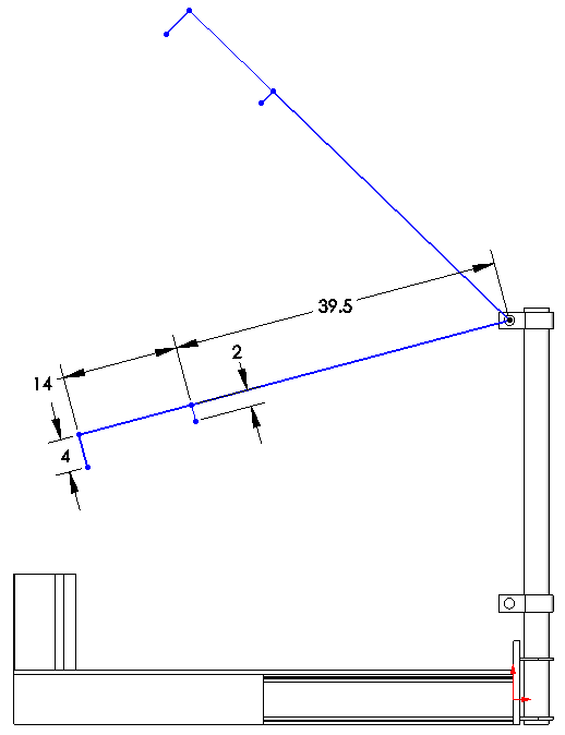
After modeling in our jib support locations, we will make a sketch. Once in sketch mode, we need to determine what our coordinate system should be. Since our jib tube is long, straight and easy to put a level on, I am choosing that as my ‘x’ axis no matter what the jib rotation is. I will then draw a line 39.5” out from the pivot and 2” perpendicular to it. This will mark the location the cylinder attaches.
Next, I will add another collinear line to the 39.5” line that is 14” long and a 4” line perpendicular to it. This is where my load chain will attach.
I will then want to duplicate this four line part of the sketch using equal length, collinear and perpendicular relations as needed, thus creating two positions in the articulation. At this point we can drag these entities into a rough position of where we want the articulation to be.
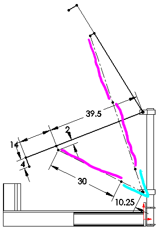
This is where it gets fun! Now we can add the cylinders in. Since a cylinder can be divided into two sections, dead length and stroke; we will draw them as two different lines. The dead length is the retracted length minus the stroke (teal). For most off the shelf cylinders, this dimension ends us being about 10.25”. The larger the cylinder you have, the greater the dead length. The teal lines represent the dead length and there is only one section per cylinder. On the lower articulation, I have one section of stroke (fuscia) and the upper articulation there is two. This will show the cylinder in the fully raised and fully lowered position.
There is a lot of time spent in this step of the process. There are so many variables to change: stroke length, 30 in; dead length, 10.25 in, the cylinder dimensions to the jib pivot, 39.5 in and 2 in. In this example, it is a fixed distance between the jib pivot and the lower cylinder mount, but it doesn’t have to be. In fact there is nothing forcing the cylinder to be mounted directly underneath the pivot either.
When designing geometry in Solidworks, an unsolvable sketch means that your geometry is bad. Reducing cylinder stroke can often rectify the situation. Also, make sure that you are able to stroke the cylinder fully without having to worry about not being in a rest or holder or unintentionally contacting other components.
Calculate the geometry, loads and forces by creating a mathematical model
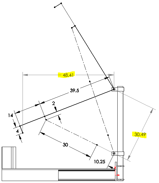
One really cool thing is that we can calculate the force on the cylinder at this point with relative ease. If we add two dimensions, we can learn the cylinder moment arm and the load moment arm.
The highlighted dimensions show the load moment arm, 48.41 in, and the cylinder moment arm, 30.49.
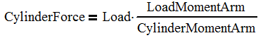
If we assume a load of 1000 lb, our cylinder load will be 1000 * 48.41 / 30.49 or 1588 lb. From here the force on the cylinder is easy to calculate:
If your load is constant, the highest load on the cylinder will either be at the minimum or maximum cylinder stroke. This just happens to be super convenient because that is what we modeled. It is not a coincidence though.
A deeper dive
So in most cases we want to know more than just the cylinder force. Things like the forces on the pivot pin and jib angle are also important. Hydraulic cylinders are generally powered by a constant flow of hydraulic oil. This means that the cylinder will extend at the same rate throughout the stroke and regardless of load on it. However, linear motion powering articulation is never a constant. Knowing the instantaneous change in articulation vs cylinder length is also important. Many times, the articulation can change far too rapidly near the end of the cylinder stroke and the system needs to be redesigned.
In order to calculate these things, we will need to take a deeper dive and use some trigonometry (breathe) to calculate the forces and lengths of all the components. Before we get to that, we need to first determine if we want an articulation based mathematical model or one based on the cylinder stroke. I see benefit both ways, but I generally fall on the side of going with articulation based. This way I can specify and angle and get the exact height and reach.

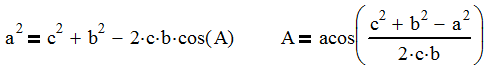
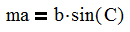
So the image above shows the mathematical representation of our geometry. We will be using the Law of Cosines and Pythagorean Theorem or Rasmussen’s Law (yeah, I proved it and named it after myself). Since we are going to use the Law of Cosines, we will first label the sides a, b, and c and the angles opposite those sides as A, B and C.
In my example, we will be defining the angle θ as the articulation angle. It is pictured here in the negative as one looking at the log splitter is most likely going to consider this a downward slope. We can quickly define θ as:
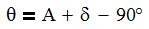
Where
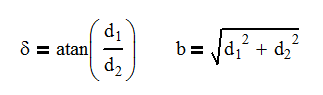
And
It is at this point that you either select to specify the angle (θ) and calculate the cylinder length (Lc or a) or specify the cylinder length and calculate the angle.
One thing to note is if the cylinder didn’t mount directly below the pivot, there would be another angle we would need to either add or subtract from the articulation equation to find θ.
So in a parametric sketch, it is easy to measure the cylinder length and moment arm with a dimension. However in a mathematical model, we just don’t have that luxury. So once again it is trigonometry to the rescue. Using the following equation, we can determine the angle, C.
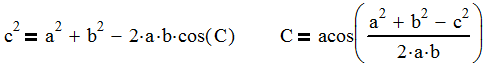
Now we can use the following equation to calculate the moment arm.
It is just that simple to get the information that you want from the model. At this point, we can start looking at the forces on the cylinder and pivot pin.

The first thing that needs to happen here is to select a coordinate system. This is a critical decision and can make calculating the forces easy or hard. In this case, I have decided to always have my jib tube be the x-axis. I do this because the angles Δ and θ are both relative to the jib tube as the tube articulates. If I choose the obvious reference frame of the jib support tube being the y-axis, I complicate the angle of the cylinder by having to combine the angles of θ and Δ as well as making the length a function of the angle θ. The other benefit of using the jib tube as the x-axis is if I wanted to operate on a slope, I can add or subtract the slope from θ.
A final note is that we will be ignoring the contribution of the 4” offset where the load attaches. The angle it adds is only 4° and not a significant enough source of error to consider it. We can easily oversize the components here to compensate.
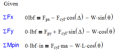
We can now perform statics on the jib tube and develop the three following equations that will specify our pin and cylinder forces:
So there are many reasons to choose MathCAD or Excel for doing this analysis. As a result, I usually do both if for no other reason, I can check my work.
The benefits to MathCAD are:
And the cons are:
The benefits to Excel are:
And the cons are:
Below is a MathCAD mathematical model where the articulation angle is specified and we can determine multiple outputs which are highlighted in yellow. One of the drawbacks to a MathCAD model is we are only able to analyze information one angle at a time. Other than that, it is quite easy to see the flow of logic.


So the first thing that I like to do in Excel is to create a sheet with only constants in it. Here is my list for this project. Under the ‘Formulas’ tab, I can define a name for each variable. When I want to use the variable, after typing ‘=’ in the cell, I can select the variable from the ‘Use in Formula’ command. This is one of the greatest features Excel has added! No longer does the formula look like $D$2*A4, but now it will display the variable name! This is a Godsend for formula troubleshooting.
The next step is to start entering data from our formulas into a different Excel sheet. Here you can see that my articulation angle is the input and the rest of the table is outputs. I basically copied the formulas from MathCAD and in some cases, rearranged the variables to solve for the intended one.
I have also put limits on the cylinder length using conditional formatting. The cell turns red if the cylinder length is less than stroke plus dead length and if it is greater than twice the stroke plus dead length. This is a helpful check to see if the articulation even falls into the range of motion that is intended. In this case, the cylinder has range from about -21° to +59°.

One thing that I love about Excel is that you can calculate and see all the information at the same time. For this reason, I will probably never abandon Excel for calculations of this magnitude. Since I can see all the data, I can produce plots like the one shown below. This is a plot of the articulation angle vs the cylinder length (blue line). I have imposed a linear trend line not only to expose the average rate of change, but also to show that the cylinder length and articulation aren’t proportional to each other.
I have also added the rate of change of the curve (orange) and you can see that as the cylinder length increases, the rate of change decreases. This is a great tool for planning your hydraulic system because it allows you to evaluate where on the curve you are planning to operate. You may find you need reduced flow or a proportional valve to help control the system.

Selecting a cylinder is usually as easy as choosing a bore, but sometimes a custom cylinder is needed for things like: load holding, special spacial considerations, position monitoring or different mounting options.
The cylinder in this case has low working pressures, so there isn’t much design work that needs to be done here. However, on larger systems where high loads demand high pressures there is need to not design up to the limits. As a rule of thumb, 94% efficiency can be expected from a cylinder. You should also plan to stay at least 300 psi below your relief valve setting. Relief valves partially open before their setting dumping some flow to tank. We want that relief fully closed in normal operation. If using a compensated valve with load sense functionality, you will want to stay at least 50 psi under the margin or standby pressure.
The reason I say this is from personal experience. Twice in my career I’ve designed a machine where the cylinders just weren’t strong enough to lift the load by just a little bit. A change in geometry was needed for both cases and it lead to smaller articulation and a cylinder redesign for longer stroke. Once your cylinder and structural design is complete and built, it is usually next to impossible to make dramatic increases to performance without going back to square one. I say this because you are less likely to get heat from a cylinder that has more capacity than you need. Error on the side of more cylinder capacity.
The final step is tweaking. Yes, you can tweak anything to death, but try to set firm limits on your design timeline. Once you have a rough layout, analyze all aspects of your design by asking some of these questions and making up your own.
If you are not satisfied with the answer to any of these questions, go back and tweak. It is so much easier to tweak the design on paper than to wait and see what happens.
This process is a difficult one for any engineer. Fortunately, we live in a time with parametric sketch technology which makes it so much easier to choose the geometry right for your application. Break the process down into the steps mentioned above and it gets simpler! Doing the process in small steps with help you master this process quickly.
In this video, Corey explains what planetary gear systems are, how to calculate speeds and their widespread use in transmissions.
It is often the case that my beam is loaded in a way that is not in a design table. So what do I do?
There are several approaches to calculate beam moments when your load case in not in a table:
I’ll explain each in greater depth.
This is by far the hardest method of calculating moments or deflection on a beam. Don’t reinvent the wheel! We are smart engineers, let’s do what we do best: make assumptions and choose one of the other alternatives.
There are a few cases where we might need to derive our own formulas. The prominent one is a case where we are interested in deflection but our beam has a tapered cross section. Another case is where we have a beam deflecting under its own weight, but it has multiple cross sections. In these cases, we will need to refer to the beam deflection equation:
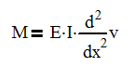
Where M is the moment, E is Young’s Modulus, I is the area moment of Inertia and v is the vertical deflection.
So….Avoid choosing this option wherever possible. The math just isn’t worth it.
Simplifying a load is often a quick work around. When I first started out as a design engineer, I sized pins by using distributed loads around cylinders and bores. This took a much longer time to calculate and lead to headaches. A few years back, a colleague challenged my approach and I’m glad he did. We both worked a few problems my way and his way. We ended up with the same results either way. Since then, I have reformed to doing it the much simpler way.
So my first suggestion is to treat point loads as point loads. I tried to treat them as distributed loads because they acted on a several inches of the beam and not just a point.
My next suggestion is to try to simplify constantly distributed loads to point loads and parabolic increasing loads to linearly increasing loads.
Many distributed loads increase, but don’t start at zero. In this case, separate the loading into a constant distribution and a linear or parabolic increasing load from zero. The magnitude of the constant distribution will be the smallest value of the variable distribution. Then subtract that value from the variable distribution.
Finally, can you ignore or combine certain loads? Often, the weight of a structure can be ignored. Or perhaps the weight can be combined with a load at (or near) the center of the beam.
Similar to the previous suggestion, oversizing a load can give quicker, but less accurate results. Often times, I am just looking for a quick go / no go calculation in a meeting and need a rough answer quickly. Oversizing a load and applying it to a known (often memorized) load case gives me the ability to give one of three answers within minutes: yes, no or more analysis is needed. As a rule of thumb, I am cautious when giving a ‘Yes’ answer. For this to happen, I generally want a design factor of over 5:1 on a ductile material. ‘No’ comes a little more freely from my lips and that is reserved for anything less than a 1:1 design factor. The ‘more analysis needed’ answer comes for things in between.
In order to quickly perform these calculations I would memorize these formulas:
Cantilevered beam with point load on end: M = P * L
Cantilevered beam with distributed load: M = w * L2 / 2 or M = P * L / 2
Simply Supported beam with point load: M = P * a * b / L
Fixed beam with point load at center: M = P * L / 8
M is the resultant moment, P is the applied point load, w is the distributed load, L is the beam length, ‘a’ is the distance from one end to the load and ‘b’ is the distance from the load to the other end.
As mentioned, this method will give you a quick answer, but the results won’t be as accurate. Please use this method with caution and always perform a more in depth calculation before proceeding with a design.
So I saved the best alternative for last. Beam calculations can be added together by using simple algebra.
Let me explain and then we will run through an example. The first thing that I will want to do is select the proper end conditions. As I apply multiple loads to my beam, they all must have the same end conditions. There are six basic end conditions that you will find tables for.
The next step is to isolate all the load cases. This could mean all point loads, distributed loads and moment loads. Each one will need to be its own load case.
Once that information is determined, points of interest will need to be determined. For a cantilevered beam, this is most likely at the cantilevered end. However, there may be other points of interest if the beam has a tapered cross section. Depending on your loads, there may be 3 to 7 points were you want the moment calculated. I typically label these points with uppercase letters and skip I, L, M, O, P, Q and R because they are already used in calculations or easily confused with numbers.
Now here is the hard step, you will need to calculate the shear and moment at each of the points you have selected for each load case. Many tables have information on the moment at key points, but you will need to find a table that has the moment as a function of the distance across the length. For example, my table for a fixed beam with an offset point load doesn’t give me an equation for the moment all the way across. It does give it to me for the length from the left support to the load, but not the other side. This can make it very difficult to find the moment for all cases on all points. I use the numbers for each load case starting with 1.
At this point, you can simply add all the Moments at each point up as follows:
MA = MA1 + MA2 +…+ MAn. Easy Peasy.
Likewise, shear forces add the same way:
VA = VA1 + VA2 +…+ VAn
And deflections too!
ΔA = ΔA1 + ΔA2 +…+ ΔAn
Once you get all these things at point A, move on to point B and C and…. You get the drift. Before I move on to an example, be sure to watch your signs. Generally speaking, point loads consider down to be positive. If you have an up load, note it with a negative (-) sign! Moment loads can also be tricky. A clockwise moment is generally positive.
One note of deflection: many cases only have the deflection for certain cases and for critical points. While you can add deflections together, it may not be worth the time to figure out what the deflection is over the entire span of the beam.
In another article, we looked at combining a bunch of loads on a traffic light cross arm. Please refer to that as an example of adding multiple sections together. I want to do another example with different supports.
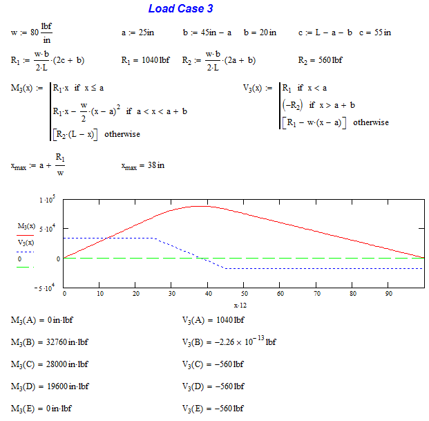
As an example, we will have a 100 in long beam that is simply supported at each end. We will put a point load of 2000 lb at 65 in, a distributed load of 80 lb/in from 25 in to 45 in and the weight of the beam at 4 lb/in.
By inspection, we can pick out a few areas of concern that we will select for calculation. First off, each endpoint will need to be looked at. For the point load it will be at 65 in. The weight distribution will be at the center, which is 50 in. The segmented distributed load is a little trickier. If using a constant cross section, we know that the deflection will be highest where the moment is highest. According to our table, that is at location a+R1/w and we will calculate that value a little later.
So, our points of interest are: A = 0 in, B = a+R1/w, C = 50 in, D = 65 in and E = 100 in. We will calculate the moment and shear force. Since A and E are reaction points, the moment and deflection are by definition non-existent, but we will calculate the shear reactions.
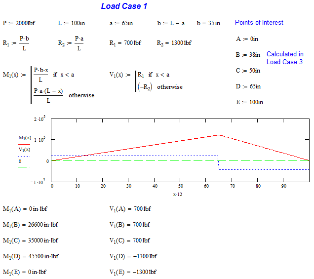
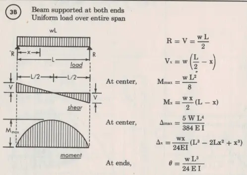
Now let’s get started. We will want to keep our three cases separate. They are shown together in the top view with points A-E labeled. Then they are separated into their individual load cases. (All table images are courtesy of Blodgett’s Design of Weldments published by Lincoln Electric. You should own a copy. Visit mentoredengineer.com/resources to buy and for other reference materials)

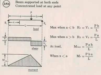
This is a simply supported case with a non-centered load. The load is 2000 lb at 65 in. The formula for the moment as a function of x, Mx, is only given from until x is less than a. To solve for this, I reversed my reference and started counting my moment as a function of y starting from the right, My. The moment equation is M = P*a*y/L. If I declare that y = L-x, I can substitute that into the original equation and get M = P*a*(L-x)/L. This is a technique that can be used in many cases and needs to be in your engineering tool belt.
Another thing to note is that the shear forces are negative on the right side. This is true, but keep in mind that the force from the reaction, R2, is upward and brings the shear force back to 0 lb. Remember to invert that force when calculating reactions.
We will now turn to MathCAD to calculate the moments and shear forces at all five points of interest. You can see that the highest moment is at point D, which is why we selected it. Also note that the magnitude of shear forces sum to 2000 lb and the moments at each end are 0 in-lb. These are good things to check for each case.
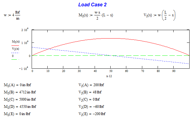
Load Case 2 is the distributed load caused by the weight of the beam. Its contribution will be minimal to the overall design and that is why this component is often ignored. The interesting thing about this loading is the shear stress is always decreasing. This leads to a constant parabolic shape of the moment curve. This load case is very easy to calculate because it is a continuous function.
When we go to MathCAD, we can see that our moment are 0 in-lb at the ends and the shear forces equal the loading of 4 lb/in * 100 in. Our highest moment load is in the center as we expect it would be.
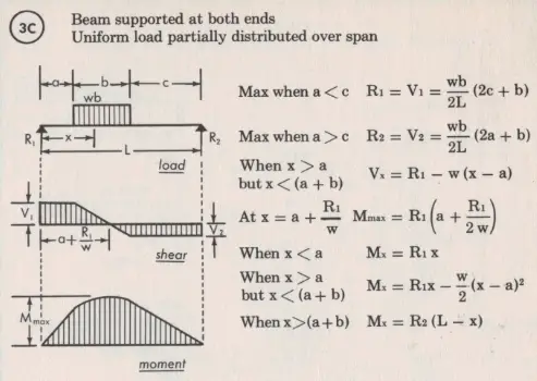
Load Case 3 is the most difficult because there are three portions of the curve that need to be analyzed. The shear stress is constant when x is less than ‘a’ or greater than ‘c’. It is linear between ‘a’ and ‘c’ and linear between the two. When integrated to get the moment, the slope will be linear up to and after the load and parabolic for the load.
I want to point out here that as the distance b decreases, the plots and formulas represent the case of a concentrated point load. Often times, a segmented distributed load can be approximated as a point load if b is small in comparison to the overall length. The moment will end up being a little higher. Conversely, if you have a large point load, you can distribute it to lessen the moment induced to the beam.
It is in this section that we will calculate location B which occurs when the moment is highest. This occurs at x = a +R1/w or 38 in.
Once again MathCAD confirms that the moment and shear forces check out at the end points. The maximum moment is at location B, just as the formula predicts and by definition, the shear is 0 lb. (If the shear force was other than 0 lb, it would indicate there was more area under the shear curve to add to the moment plot)
The last step is to sum all the individual components together and determine where the maximum load is. In this case, point D has the highest moment load and near the highest shear load. This would be the prime candidate for structural analysis. Now, it looks like there may be multiple locations to check for high stress. If you have a shear plot, we can see where the shear load is above or below 0 lb. If it is above, moment will continue to increase. Once it turns negative, moment will start decreasing. In this example, the shear load does not cross 0 lb until 65 in. This way we know that this is the maximum load point.

Well, beam analysis is a tough subject. As you can see from the graphs above. There is no loading case on earth derived for is case. There are many ways to approach a beam loading that is not in any tables. The easy way is to combine simpler loadings from the tables into a more complex one. An even easier way is to use my beam calculator have it do all the work for you.