I often get the question of what type of roller chain should be used in an application. Let’s unpack that question in this article.

A standard duty roller chain should be specified unless spacial constraints prohibit the use of a larger or double chain. Selecting a standard duty chain allows for the opportunity to increase in strength if needed by converting to a heavy duty or double row chain later.

If you know me at all, you know that I always like to have a Plan B in mind. If something isn’t working right, I will work on it to a point, but I always want to have a backup design ready.

I am no different with roller chain. If I design to standard duty roller chain, I have three different options immediately available when (er…I mean if) it isn’t working correctly. They are

• Heavy duty chain
• Multiple strand chain
• The next pitch size up

Before we dive deeper, we need to gain a little knowledge in the components of a roller chain link. Click here to see a video on how roller chain is made.

Roller Chain Components

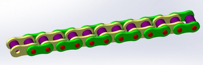
The main parts of a roller chain are the inner and outer links, pins, bushings, and rollers. The bushings are rolled plates that are pressed into the inner links which are the dogbone shaped plates. The roller is inserted over the bushing before the second inner link is pressed on. Next, the pins are pressed into an outer plate. Then two inner link assemblies are assembled over the pins and the second outer plate is added. The ends of the pins are mushroomed in the pressing step so that the link will stay together. That was all in the video, you should have watched it.

Please note that smaller chains, line the one shown below, do not have a bushing under the roller. This is because the bushing would be rather small and difficult to handle.

Designation of Roller Chains

Roller chain has an interesting designation system. The last number in the designation can be 0, 1 or 5. A 0 designation is the standard roller chain as described above. A 1 designation refers to a narrower variation of the standard, 0, configuration. A 5 designation refers to a chain without a roller.

The first one or two numbers of a roller chain refer directly to the chain’s pitch. To get the pitch in inches, divide the number by 8. If you desire millimeters, multiply by 3.175. For example, a 50 chain has a pitch of 5 / 8 or 0.625″. For metric, 5 times 3.175 is 15.9mm.

Chain is usually sold in feet, so it may not be critical to know exactly how many links are needed. However, in critical applications, the tensioning device may not be able to handle too many or too few links. If you want to know the number of links, you simply divide the length needed by the pitch.

Standard chain sizes are 25, 35, 40, 41, 50, 60, 80, 100, 120, 140, 160, 180, 200 and 240. For single rows of chain, you will see the chain specified as 50 or 50-1. If two or more rows of chain are needed, the chain will be specified as 50-2 or 50-3 etc. If a heavy duty chain is required, a chain designator of ‘h’ is added to the end (i.e. 50-1h).

A heavy duty chain will use stronger components made of better grades of steel than a standard duty chain. A different heat treatment is also applied to increase strength. Finally, the link plates are usually slightly thicker. All this is to say that you will only get an incremental improvement in performance.

The pin is usually the weakest component in the link and there is only so much that one can do to increase its strength. A pins greatest weakness is bending loads and chains are designed to minimize that, but as the shear load goes up, the bending load goes up exponentially. In fact, just having thicker plates makes the bending load on the pin go up.

Chain Strength

Manufacturer’s literature may have the chain’s strength listed as the tensile or breaking strength.

Do not design to the tensile or breaking strength!

The breaking strength is the amount of load that the chain can handle before breaking. That’s failure! It does not account for manufacturing tolerance, chain wear, misalignment, shock loading or twisting. We should design to the working load!

As engineers, we design to the working load, which for roller chain is a design factor of 8:1. You may want to increase or even possibly decrease this factor based on your application. Shock loading is probably the largest driver in choosing a design factor.

Below is a table of typical chain breaking strength values and the relative cost to a 25-1 standard chain. While this table is not thorough and exhaustive, it will give you the tools to make informed decisions for your application.

Chain Size	Standard Breaking Strength (lb)	Relative Cost to 25-1	Heavy-Duty Breaking Strength (lb)	Relative Cost to 25-1
25-1	930	1.00	1010	2.04
35-1	2320	0.76	3920	2.04
40-1	3970	0.88	5181	2.42
50-1	6260	1.16	7940	2.46
50-2	13230	2.64
60-1	9270	1.51	12130	2.05
60-2	18530	3.56
80-1	16540	2.67	19850	3.43
80-2	33080	5.73
100-1	25360	4.32	30870	5.76
120-1	32640	6.32	36390	8.32
140-1	45210	7.78	48510	10.23
160-1	57780	9.74	60630	13.13

One thing that is almost immediately visible is the 35-1 and 40-1 chains are cheaper than a 25-1 chain. This probably has to do with two things. First, the 25-1 chain isn’t very strong so most people probably don’t use it. Second, the parts used in the 25-1 chain are small and require more handling and that leads to less production. If you are already considering moving away from a 25-1 chain, just go to the 35-1. You won’t regret it.

In all but a few cases, you will get more bang for your buck by moving up one chain size. This move dramatically improves your strength, with a minimal impact to cost. The most notable improvement of 149% increase is going from 25 to 35 chain at a cost savings and the next would be going from 35 to 40 chain for a 71% increase in strength.

In fact, the only cases where going from a standard chain to a heavy duty chain is for 60, 80 and 100. On the 60 chain you get 24% more strength for 36% more money. With 80 chain you get 17% more strength for 29% more cost. Finally, with 100 chain there is a 18% increase in strength at a 33% cost increase.

While these numbers are representative, you might be able to find better deals than I can. The last major observation is that there wasn’t a case where it made sense to switch to a double or even a triple chain.

Why upgrade to a double or triple strand roller chain?

Good question. There are a lot of good reasons to upgrade to a multiple strand roller chain. Let’s look at a few.

• It doubles (or triples) the working load easily. There isn’t a need to fully redesign an existing system. Sprockets and chain guides are usually available in single and double strand configurations
• Your design has height constraints, but can be widened.
• Your sprocket needs to have a certain number of teeth. Increasing the tooth count may throw off running speeds unless all the other sprockets are increased accordingly. Also, a sprocket for the larger chain size may not be available in the same bore.
• Since there are two or more strands, there should be better wear and less friction between the chain and sprocket. This assumes that the chain is not misaligned.
• The chain will have a longer life

How to upgrade

So you’ve made the decision to upgrade your chain from a standard chain to heavy duty or a multiple strand chain. It is very important before any parts are purchased to check the design calculations. If your calculations are good, but you are having issues with chain breakage, something else is in play. My guess is there is misalignment, interference or a shaft that isn’t rotating freely. Please see my guide to preventing roller chain failures.

The next step is to examine every part of the design in 3D CAD (if possible) and in real life to identify the possibilities of rubbing, pinching or even if extra chain support is needed.

If you do nothing else, make sure that you can assemble the machine with the wider chain and sprocket. This is one thing that most young engineers will forget about. This causes headaches all around.

You will also need to investigate increasing the tensioning devices for your chain. The weight increase of a heavy duty chain is minimal, but going from single strand to double or triple strand will double or triple your chain weight. You need to be prepared for this

Pay special attention for misalignment. When going to multiple strand roller chain, it is often the case that alignment tolerances have been eaten up with the wider sprockets.

Finally, when upgrading to heavy duty roller chain, you need to make sure that all the chain components are heavy duty rated. The most overlooked components are the connecting links.

Conclusion

From our investigation into what roller chain type we should be using to design to, we have found that the standard single strand roller chain should be used. In almost all cases, increasing the chain to the next pitch size gives us the most improvement in strength for the least cost. We also looked into reasons why we would use a multiple strand chain.

Finally, be sure that when you change your roller chain for an existing application that there is plenty of room to assemble the larger sprockets.

Roller chains are great ways to transmit power. Like all power transmission, there are certain rules that need to be followed. This article should give you insight into selecting the right roller chain.

Springs are essential to life.  In fact everything on the planet acts like a spring, which follow Hooke’s law.  When force is applied to an object, it will deflect.  If more force is applied, it will deflect more. 

When designing or selecting a extension spring you need to consider: the spring shape and end type, the number of coils, the preload and allowable stress, the spring index. You can then calculate the stress on the spring using one of five basic approaches.

One crucial thing to understand when designing extension springs is to be sure to operate them in their intended range.  All springs work well in their linear range, but as soon as they are loaded past the yield strength, the spring stops behaving as intended and the spring life is severely shortened. 

Furthermore, the consequences with an extension spring are much higher. When a compression spring fails, the pieces are still in a bore or around a shaft and the components remain in contact with each other. If an extension spring fails, the components will be separated from each other and the result could be disastrous.

To illustrate this, if a spring in your cars suspension fails, your car will still be in one piece and you could at least make it to the side of the road before too much damage was done. On the other hand, if your trampoline is missing too may springs, you are falling through to the ground.

One of the most fascinating things about springs is that the method they are used in is opposite of the load they see.  A compression or extension spring is loaded in torsion and a torsion spring is loaded in bending.  I liken this to tightening a hex head screw with a socket wrench and tightening a socket head screw with a hex wrench. It’s all backward!

1. Spring Shapes

Cylindrical extension springs with hooks on the end are by far the most common type available, but there are other shapes to consider.  The most popular are:

• Swivel Hook
• Straight Cut
• Drawbar

Cylinderical Hooked Springs

Cylinderical springs are very common and come in a variety of sizes as an off the shelf part.  The OD and ID of the spring is consistent for the length of the spring coils they are generally intended to be hooked on each end.  The spring rate is constant once preload is overcome (more to come on that). Adding extension springs in series will enable more travel, while adding them in parallel allows for more force.

One important thing to note with hooked springs is that the highest stress is at the ends of the spring. You can see that the two spots where the spring is first bent to start the hook is where the stresses are the highest. Typically the hook is formed in at least two moves so that the increase in stress is minimal.

Swivel Hook

            Swivel hook extension springs are rarely used. This spring is a barrel spring coiled around a hook on each end. This design is more expensive but it does deal with the higher stresses at the end of the spring. The main benefit is that the ends can pivot so that if the end mounts aren’t in line additional stress on the spring is not added.

Straight Cut

Straight cut extension springs are like regular compression springs, but wound so that it is an extension spring. The main benefit of this is that springs can be ordered in long stock lengths and cut to the desired length. This allows the engineer to get the spring characteristics desired quickly and without purchasing multiple springs.

Terminating these springs is very unique. The spring comes in diameters that match available threaded hardware. These springs are terminated by threading a fastener into the spring. This allows you to have a complete control over terminating with a capscrew, eyebolt or hook. The sky is the limit. Just make sure that you subtract the engagement between screw and thread in your calculations.

Draw Bar Spring

Drawbar springs are a way to use a compressive spring in an entension spring fashion. The main benefit is that the drawbar sits inside the spring and prevents the possibility of the spring failure separating the components at each end. (However, the drawbar could still fail is loads are high enough.)

Drawbar springs are used in winter pool cover attachment, porch swings, porch doors, trampolines and any application where if the spring fails, the components need to stay attached.

Many people use these to tie off a boat so that if the spring breaks, they don’t have to go searching for their boat.

2. Extension Spring End Types

There are three basic types of extension spring ends, they are:

• Machine Hook
• Machine Loop
• Double Full Loop

These spring ends are easy to identify when shown next to each other. A hook end will allow an object to reach around the end of the hook to engage. Generally speaking this allows the hook to engage and disengage without disassembly.

The loop configurations are closed so assembly usually requires it so stretch over an object and another part to secure it. Imagine that the spring stretches over the end of a threaded rod and a lock nut is added to hold it on.

A double loop end is used when strengthening of the loop is needed. If the spring was loaded laterally, there might be enough force to open the loop on a single machine loop end. The double loop prevents this.

Other end types that are less popular are

• Full loop on the side
• Offset hook on the side
• V-Hook
• Elongated Round Hook
• Small loop on the side
• Small extended loop

If none of these fit your fancy, you can create your own custom spring. They can pretty much make any end design to your specifications.

One other consideration for the end condition is the angle of the loops, hooks, or whatever you thought of is one end’s relative position to the other end. An off the shelf spring will have the ends in line. They assume that you are linking things together like you would a chain. You can specify if your spring should be inline, perpendicular or random. Random, of course, gives you the lowest cost, but the least control of your design. If you are willing to foot the bill for a custom spring, you can specify any orientation you would like.

3. Number of Coils

Unlike a compression spring, counting the number of coils on a spring is straight forward.  The only exception is the drawbar spring so you should consult the compression spring design guide. Most extension springs are designed with a preload and that will manifest itself with the coils touching each other.

Start counting each coil from one end to the other starting where the first overlap is. Keep counting until you get to the other end of the spring. Generally speaking, coils are counted as full turns, but half and quarter turns are also widely used. Many spring manufacturers will allow two digits of precision on the number of coils.

4. Spring Preload

Extension springs are able to have a preload in the design. This allows a spring to have some load at no deflection. This idea has a parallel in fastener design because they both rely on Hooke’s Law. A fastener is torqued to a load higher than the design anticipates so that it will not be subject to fatigue.

The preload on a coiled spring comes from several, if not all of the coils being twisted so they want to be on top of each other. It is basically adding a torque in the opposite direction of the spring.

Theoretically, the spring will have no deflection under load until the preset tension is reached. After that it will follow the linear spring rate. However, when the load is right at the preload, the load-deflection curve will make a smooth transition instead of a sharp curve. This generally isn’t the part of the curve that we are working in so it usually is ignored.

This phenonemon is caused by unequal twist in the spring coils. The theoretical case is that all of the coils separate at the same time. In reality, some coils with separate first and others won’t.

The above chart is zoomed in so that the theoretical vs actual curves can be distinguished. When the chart is zoomed out, the magnitude of the preload effects can be seen in proportion to the rest of the springs working envelope.

5. Allowable Spring Stress

All springs function according to their dimensions.  The dimensions will specify the stresses seen in the spring.  Based on general stress calculations, we know that the largest stresses in a extension spring will be on the outside surface of the wire as load is applied. 

When designing a spring, the dimensions are critical to spring characteristics.  Often we are confined by the form factor where the spring is applied, i.e., the spring needs to fit in a ¾” hole or over a ½” rod.  As the designer, if you find that there is only one or two choices for springs available, you may want to ask yourself if you are being too strict with the design.  I have often found that in my design I needed to go up in capacity, but the form factor was already set in stone.  Now it is really hard to get the performance I need.  Had I adjusted my design to have four or five choices of springs, I could simply change out a spring.  In practice, I desire to have five choices; my ideal spring plus two stronger and two weaker spring alternatives.

The life of the spring is dictated by fatigue.  As the spring is cycled, grains in the steel rub against each other.  As they repeatedly rub, small cracks will get larger and larger until failure occurs.  There are two main components that dictate the life of a spring; the number of cycles and the stress intensity.

The number of cycles is pretty easy to determine, it is something that is easily counted or estimated.  We find that most materials have an endurance limit, where if the spring makes it to that number of cycles, it will last forever.  For steel, this occurs around 1-2 million cycles.  Unless your spring is custom, vendors only make springs with infinite life.  Even then, vendors will fight you on a finite life spring.

Stress intensity is much more complicated.  A lot of it has to do with the mean (average) and alternating stresses.  The average stress, alternating stress and stress range are defined by the following equations.  We will use a maximum stress of 50 ksi and minimum stress of 10 ksi.

Since we are only dealing with extension springs, the minimum stress is usually zero unless the spring has a preload. In this case, the preload would be a negative stress.  In the case above and after the spring is installed, we will always have a preload on our spring.  This is usually the case in applications like a gas motor where the carbeurator needs a minimal amount of force to keep a valve open or shut.  We want preload on it so that the valve doesn’t vibrate when at rest and it also requires some force to move. 

In any case, our stress range is 40 ksi.  To extend our spring life, we will want to decrease this as much as possible.  If an extension spring was to have an initial preload, the minimum stress would be negative thus increasing the stress range greatly and decreasing life span.

One step that spring manufacturers perform to limit the magnitude of stress is to stress relieve.  The stress relieving process heats the spring to high temperatures so that permanent or residual stresses from the forming process are eliminated.  The temperature here is not so high that the spring would lose its initial temper.

When designing an extenstion spring, a fairly conservative design factor is used. THis is mostly because of the heightened risk for catestrophic failure if the spring fails. The stresses are generally less than 60% of the materials tensile strength.  Sixty percent is chosen because the endurance limit of most materials is around 60% of tensile strength. 

6. Spring Index

The spring index is a simple ratio of the mean diameter to the wire diameter.  It is a variable used in many spring calculations and give us an idea of what type of spring it is.  The index should be kept between 4 and 10. 

If it is lower than 4 and your spring is coiled too tight, this will require special tooling to form.  When forming a tight radius, you might also have problems with the material cracking internally and that will lead to premature failure. 

Spring indexes greater than 10 means the spring will be real flimsy and lead to problems with packaging and tangling.  Think of a slinky.  You also won’t be able to grind or perform other operations like plating. 

This should be a giant red flag that something is not right with your design.  Don’t design yourself into a hole!

7. Spring Calculations

So this is a little bit of a backwards approach.  There are five main ways of selecting a spring, but they only make sense once you understand the equations behind spring design.  For this we will go through the calculations and then come back to the methods of selection.

Most spring design is done based on dimensions so it is likely that you will have the outside diameter (OD) and the wire diameter.  From these two pieces of information, we can find the inside diameter (ID) and the mean diameter, D_m using the following equations:

From here we can calculate the shear stress on the spring coils (assuming the wire is round).

Where C is the spring index, P is the applied load and K is the stress concentration factor.  Note K is shown for extension and compression springs.  Other types of springs have different values.

Because of the radii needed to form the hook or loop, we also need to calculate the stress in both areas indicated below. Points A and B will be calculated with the formulas below.

To calculate the normal (bending) stress at point A, use the following formulas.

To calculate the shear stress at point B, use the following formula.

Once all these are know,n, the coil shear stress and the shear stress at point B will need to be summed using the square root of the sum of the squares. If you want to convert the shear stress to normal stress, use the maximum distortional energy theorum as a conversion. You will divide the shear stress by 0.577. (See the Mohr’s Circle Video for more information on this.)

The final step is to calculate the spring rate, R

Where G is the shear modulus of elasticity and δ is the deflection.  Many times you will be given the spring rate, so we can rearrange this equation to calculate the number of active coils in the spring.

8. Spring Selection Approaches

There are five basic methods for selecting a compression spring.  You will need to select one of the five that best fits your application. 

1. Design based on physical dimensions
2. Design based on spring rate
3. Design based on two loads
4. Design based on one load and spring rate
5. Design based on one load and free length

Case 1: Design based on physical dimensions

This is probably the most common method of designing a spring.  When approaching the design you probably already have a certain envelope that the spring must fit into or around.  When selecting a spring by physical dimensions, you need to specify two of these three things:

• Outside Diameter – OD
• Inside Diameter – ID
• Wire Diameter – d

Case 2: Design based on spring rate

When you know the spring rate you desire, you can start your selection there.  You will need other information such as free length, load capacity or some dimension of the spring to complete the selection.  Once you have selected this information you will probably be able to calculate the number of active coils and the free length using the following equations.

Case 3: Design based on two loads

For this design criteria, you will specify the spring rate based on two loads that are applied to the spring.  At each load, the spring will deflect differently.   Many spring manufacturers will have this option of choosing a spring on their website.  The variable, L, is the total height of the spring and not the deflection.

Once you have the rate, you are basically back in the previous design case (Case 2) and need to make other decisions to select your spring.

Case 4: Design based on one load and spring rate

This is really another subset of load Case 2.  The only difference is we will be able to calculate the free length without making any other selections.

Case 5: Design based on one load and free length

This is really just a subset of Case 3 where we assume that P₂ is 0 lb and L₂ is the free length.  Then use the equations in Case 2.

So let’s run an example

I need a spring that will sustain a load of 40 lb and a maximum load of 100 at 0.50 more deflection. We can start by using Case 3 above to determine our spring rate.

Since my maximum load is 100 lb, I want a spring that has 10% to 20% more capacity than needed.

Looking through the list, I immediately notice that there is only one option of spring. My design criteria is too tight! Nevertheless, we will run with the calculations to prove they work.

At this time, I will perform my hand calculations (left) and determine the results.  I have also displayed the additional information from the manufacturer (right).  Notice how my calculations match with the manufacturer. 

At this point, we can move on to the stress calculations for this spring.  Since we are using music wire, we will assume that for this diameter, the tensile strength is 250 ksi.

As you can see from the stress calculations, the intended load is only 53.6% of the tensile strength.  If you are curious as to where the 0.577 comes from, please watch the video on Mohr’s Circle.

As we calculate the stress aat points A and B, we can see that these are also in line with our design limit of 60% of the tensile strength. The stress at Point A is 5% higher and that is why extension springs tend to break in this location.

Stress at Point A

Stress at Point B

Some Verification

Just to prove that these calculations are correct, I ran an FEA of this spring. Let’s compare the difference.

It is pretty amazing how accurate these calculations were to the FEA results. Yes, you can trust this process.

Conclusion

Spring design seems complicated because there are so many different ways to approach it.  Just remember that there is no perfect solution for your application.  With all the off-the-shelf sizes, shapes and materials to choose from, you will select a very good spring for your application.  Just remember to watch for the red flags of improper spring index and always have plenty of alternative springs ready.

You got this!

Glossary of Terms