

Beam tables give information on and assume that the deflection calculation is based on a constant cross section. So, what do we do if our beam has a cross section that changes over the length of the beam?
To determine the amount of deflection in a variable cross section beam, you must integrate the beam deflection formula with the moment of inertial being a variable with respect to the length and apply boundary conditions. The beam deflection formula is v’’ = M(x)/[E*I(x)].

Continuous or Discrete – There are two types of beam sections, continuous and discrete. Most beams are continuous beams and have either a constant section or a section that changes gradually over the length of the beam. Roof beams in large steel buildings are a great example of a continuous variable beam. The beam is relatively short in height on the ends and very tall in the middle.
Discrete beams are beams that have sudden discontinuities in the section. Believe it or not, these are sometimes easier to calculate because the discrete sections are usually constant which leads to easier calculus.
The beam deflection formula is a universal formula that allows for the customization of multiple loadings and beam sections. I will warn you that the more exact your calculation needs to be, the harder the math will be to do. Simplification here will save a lot of time and effort. As mentioned before the formula is:
v’’ = M(x)/[E*I(x)]
Where v’’ is the second derivative of deflection (the acceleration of the deflection), M is the moment which is usually a function of the position along the length of the beam, x. E is the modulus of elasticity and I is the area moment of inertia of the beam. All tabulated beams will consider this to be a constant and therefore none of the deflection formulas can be used.
Now when we integrate the equation above, we will be doing an indefinite integral which means that we have to add a constant, Cn, to the polynomial each time we integrate. Since we will be integrating the equation two times, we will end up with two constants. If we have a discrete case, we will have two or more equations.
Boundary conditions are requirements that the beam deflection formula will need to abide by when it is in the final form. The final form only comes when we use the boundary conditions to solve for the constants formed by the indefinite integral. Common cases are the ends of a simply supported beam need to be 0 (in, mm etc.) or the slope of a cantilever beam needs to be 0 radians.
In this article, we are going to walk through three examples of common variable cross section beams.
- A two-section cantilever beam with point load on the end.
- A two section simply supported beam under its own weight.
- A constantly changing continuous simply supported beam with a constant distributed load.
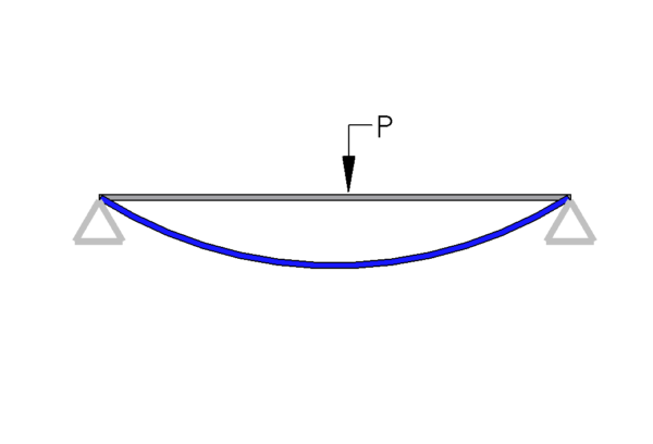
Example 1: A two-section cantilever beam with point load on the end.
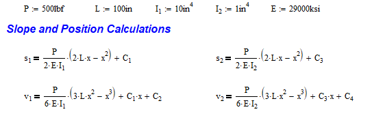
This problem with consist of a 100 in. long cantilevered steel beam with a load of 500 lb. on the end. The first 50 inches of the beam will have an area moment of inertia of 10 in^4 and the remaining beam will be 1 in^4.
Now we will determine the moment and integrate the beam deflection equation twice each time adding a variable for the indefinite integral. I have selected to make my coordinate system (x variable) start from the base. This makes the integration slightly harder, but the variables C1 and C2 will cancel out because of boundary conditions 1 and 2. You’ll see in a second.

I only need to do the integration for one of the sections and then change I1 to I2 in the equations. I have also kept the variable ‘v’ as the deflection of the beam, but changed the first derivative of deflection to the variable ‘s’, to indicate slope. I also specified the variables.
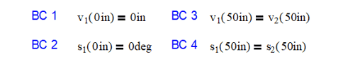
Now that the problem is defined, let’s setup the boundary conditions. We will want the position and slope at the fixed end of the beam to be 0 in and 0 radians. We will also need two more boundary conditions at the joint between the segments. The slope and position at this position will need to be the same.
Let’s solve for Boundary Conditions 1 and 2
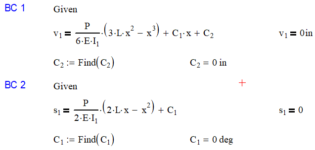
As mentioned above, I foresaw that variables C1 and C2 would be equal to 0 when I chose to have the coordinate system start at the base.
Next, we will look at boundary conditions 3 and 4. These are slightly more complex.


Please note the check that I put in the Find block so that we could verify that the v1 = v2 and s1 = s2 at 50in. This verifies that the position and slope will be continuous at this point.
The next step is to verify the results. This is done in two steps. The first is to plot each segment over the entire length. We looking for the four boundary conditions to be met. As you can see, the lines intersect and are tangent at 50 in. Also, v1 has no deflection or slope at the base.

Finally, we will merge the two plots together forming the final equation for the deflection of our cantilevered beam.

As you can see, the deflection rapidly increases once past 50 inches from the base. This is clearly indicated in both graphs.
The Best 4 Ways to Improve Torsional Beam Performance
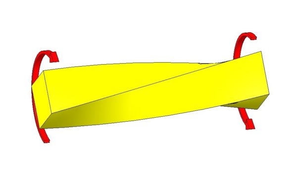
Example 2: A two section simply-supported steel beam under its own weight.
This problem with consist of a 300 in. long simply-supported steel beam with a distributed load of 30 lb./in on the left end. The right end has a distributed load of 50 lb./in. The first 200 inches of the beam from the left will have an area moment of inertia of 10 in^4 and the remaining beam will be 1 in^4.

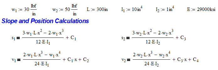
Now we will determine the moment and integrate the beam deflection equation twice each time adding a variable. I have selected two coordinate systems. The x coordinate goes from left to right and the y coordinate goes from right to left. They are related by:
y = L-x
I have chosen this coordinate system so that C2 and C4 will cancel out when we solve for Boundary Conditions 1 and 2. It also simplifies the math tremendously. You’ll see in a second.
I only need to do the integration for one of the sections and then change I1 to I2 and w1 to w2 in the equations. For the right-hand section equations, I will also substitute ‘y’ for ‘x’. I have also kept the variable ‘v’ as the deflection of the beam, but changed the first derivative of deflection to the variable ‘s’, to indicate slope. I also specified the variables.
Now that the problem is defined, let’s setup the boundary conditions. We will want the ends of the beam to be 0 inches of deflection (BC 1 and 2). We will also need two more boundary conditions at the joint between the segments. The slope and position at this position will need to be the same where the segments join.

Let’s solve for Boundary Conditions 1 and 2
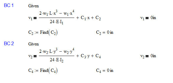
As mentioned above, I foresaw that variables C2 and C4 would be equal to 0 when I chose to have the coordinate system start at the base.
Next, we will look at boundary conditions 3 and 4. These are slightly more complex.

Please note the check that I put in the Find block so that we could verify that the v1 = v2 and s1 = s2 at 200in. This verifies that the position and slope will be continuous at this point.
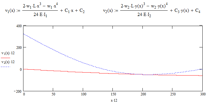
The next step is to verify the results. This is done in two steps. The first is to plot each segment over the entire length. We looking for the four boundary conditions to be met.

Uh-oh, what happened!? The lines definitely intersect at 200 in and each end has 0 inches of deflection, but they are not tangent at the intersection. Not only I am illustrating the power of graphing the solution for accuracy, but also demonstrating that using the two different coordinate systems posed a problem. According to the equations, the slopes approach the location of the junction on a downward slope equal in magnitude. However, to make this work one of the slopes actually needs to be coming up. We can fix this issue by making one small change.
s1 = -s2
Let’s make this change and proceed with the solution.

Yes, much better! Finally, we will merge the two plots together forming the final equation for the deflection of our cantilevered beam.

As expected, the longer stiffer section deflects less.
How to Calculate Beam Data When Your Case Isn’t in a Table
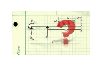
Example 3: A constantly changing, continuous, simply-supported beam with a constant distributed load.
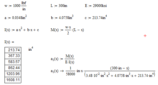
This problem with consist of a 300 in. long simply-supported steel beam with a distributed load of 1000 lb./in across the beam. The section starts off at a height of 10 inches increases linearly to the center where it reaches a height of 24 inches. It then tapers back to 10 inches.

To determine how the moment of inertia changes with respect to x, we will model in Solidworks and take sections every 30 inches. We will tabulate this data and fit a line to it.

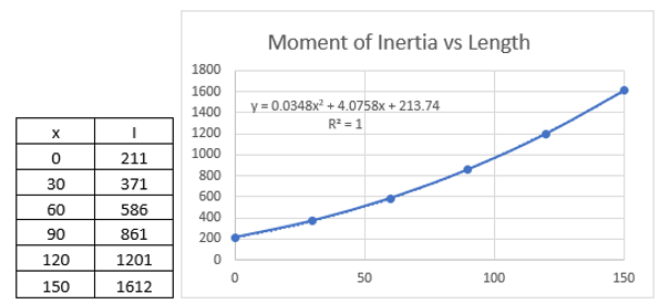
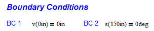
Now, you probably noticed that I only made the table for values of 0 in. to 150 in. This is because I am going to use symmetry to simplify this complex problem. We can use symmetry because both the load and beam section are symmetric from the midpoint of the beam. Because of symmetry we will need to have the end point have a deflection of 0 in and the slope at the middle of the beam be 0 deg. We can then mirror this to get the continuous deflection of the beam. For this case, we will have the x coordinate go from left to right.
You can see here that the calculated values of I(x) closely match what is listed in the table above. I have named the second derivative of position ‘a1’ (acceleration). As you can see, with the top and bottom having the variable ‘x’, it will be super fun to integrate this. So, there is one thing you need to know about me. I have limits as to things I won’t do. Integrating this is one of those things. That’s why we have MathCAD!
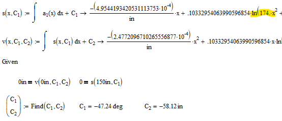
As you can see, the very tedious work of integration was glossed over and we were able to directly solve for our boundary conditions. In the equations of s(x) and v(x), there were actually natural logs and somehow an inverse tangent appeared (not shown). I’m still not regretting letting MathCAD do the work.
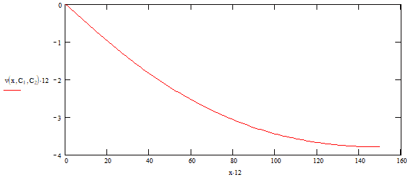
The next step is to verify the results. This is done in two steps. The first is to plot each segment over the entire length. We looking for our boundary conditions to be met. As you can see, the deflection at x = 0 inches is 0 inches and the slope appears to be flat at x = 150 inches.
Finally, we will mirror the plots together forming the final equation for the deflection of our cantilevered beam.
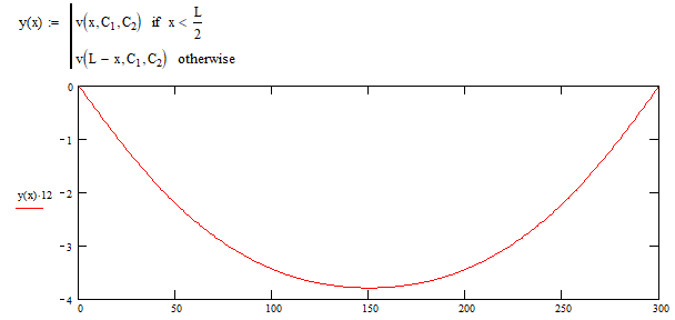
As you can see, the deflection is 0 inches at the end points and has the maximum deflection at the center.
The Best Guide to Solving Statically Indeterminate Beams
Conclusion
This article covers three popular load cases where a beam has variable cross sections. While this does involve calculus, it is often very easy to do by hand because it is polynomials. If not, be thankful for robust programs like MathCAD to perform this for you. This article should give you a good handle on the procedure used to analyze beams like this. If your beam isn’t loaded exactly like this, you can always find the moment calculation in a table and integrate your heart out.